Lesson 6-2 · Weights in the Graph
Lesson 6-2 · Weights in the Graph
Teacher mode is on. Toggle it off (bottom-right) to preview the student view.
You have a weight. Now the program needs it. This lesson starts a new section of
robot.py with a list of slow segments next to the blocked list, a weight() function
that answers "what does this edge cost?", and a path_cost() that adds a route up —
and then adds cost to the Module 5 harness as one more thing it checks. BFS,
unchanged, fails that check. On screen, with the path printed, before any robot is
involved. That failure is the reason the next lesson exists.
Learning Objectives
By the end of this lesson you will be able to:
- Store slow segments as
(a, b, cost)entries and add one withadd_slow_edge() - Write
weight(a, b)so it returns the slow cost in either direction and 1 otherwise - Write
path_cost(position, path)by walking the path and summing weights - Write
check_cost(), the cost check, and explain what its FAIL line means - State BFS's limitation precisely: it minimizes steps, and cost is not steps
This lesson's skeleton
Paste this into robot.py above RUN. It starts the WEIGHTED GRAPH section: one
list, five function outlines, no tests yet — you'll write those as you go, as you did
in Module 5.
# ===== WEIGHTED GRAPH =====
# The grid with a cost on every edge. A normal block costs 1;
# a slow segment costs what you measured in Lesson 6-1. The
# slow list is kept the way GRID GRAPH keeps BLOCKED, and
# weight() is the one question every planner asks of it.
# path_cost() adds a route up; check_cost() is a sixth
# property for the BFS PLANNER's harness, and BFS fails it.
SLOW_EDGES = []          # (a, b, cost), one per slow segment

def add_slow_edge(a, b, cost):
    """Record the segment between a and b as costing cost."""
    pass

def clear_slow_edges():
    """Empty SLOW_EDGES in place, as clear_blocked() does."""
    pass

def weight(a, b):
    """Cost of driving from a to b: the slow cost if that
    segment is in SLOW_EDGES, in either order; otherwise 1."""
    pass

def path_cost(position, path):
    """Total cost of driving path from position: the weight
    of every segment, starting with position to path[0]."""
    pass

def check_cost(test_name, start, destination, path, expected_cost):
    """Print PASS if path costs expected_cost, else FAIL with
    the cost and the path; return True on a pass."""
    pass
A second list, next to BLOCKED
Module 5 kept the things the planner needs to know about the grid in one list,
BLOCKED, fed through add_blocked() and emptied by clear_blocked(). Slow segments
get the same treatment: SLOW_EDGES, fed through add_slow_edge(), emptied by
clear_slow_edges(). Both of those are one-liners shaped like their Module 5 twins.
A slow segment is a property of the edge between two intersections, not of either
intersection, so each entry holds both ends and the weight you measured:
add_slow_edge((0, 1), (0, 2), 5) appends the tuple ((0, 1), (0, 2), 5).
Then one function answers the question every planner will ask: weight(a, b). It
loops over SLOW_EDGES looking for the pair, and returns 1 if it never finds it. Read
the docstring's "in either order" carefully. The robot might drive the segment from
(0, 1) to (0, 2) or from (0, 2) to (0, 1), and it's slow both ways, so the test inside
the loop has to match the pair either way round — that's an or of two comparisons.
Anything not in the list costs 1: a normal block.
SLOW_EDGES holds ((0, 1), (0, 2), 5). What do weight((0, 2), (0, 1)) and weight((1, 1), (1, 2)) return?
Adding up a route
A path from the planner is a list of intersections to drive to, not including the start. Its cost is the weight of every segment driven: from the start to the first step, from that step to the next, and so on.
So path_cost() keeps a running total and a here that starts at the robot's
position and moves forward one step each pass — the same shape as drive_path()'s
current_position = next_pos. For [(0, 1), (0, 2), (0, 3)] from (0, 0), with the slow edge
at 5, that's 1 + 5 + 1 = 7.
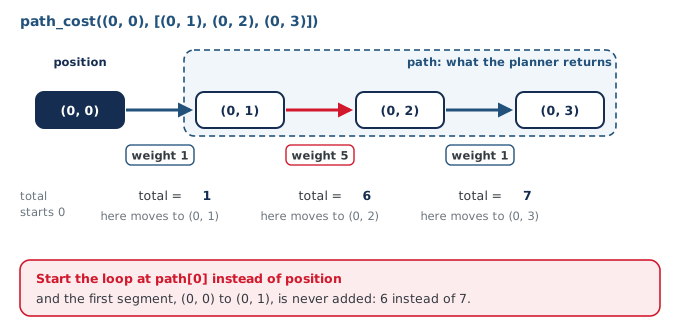
Why does path_cost() need the position parameter, when the path is right there?
The sixth property
The Module 5 harness checks five properties of a path. Add a sixth: the path's cost equals the cheapest possible. For now you work out the cheapest by hand — trace the routes on the grid and add them up — and type the number in; the next lesson writes the planner that finds it.
check_cost() is shaped like Lesson 5-6's run_no_path_test(): it prints a PASS
line or a FAIL line in the same format and returns True on a pass, so that the
harness can count it. The one difference is that it is handed the path, not the
planner, so you can point it at any planner's answer. A PASS line and a FAIL line as
they should look:
  PASS  open grid  [(0, 1), (0, 2), (0, 3)]  cost: 3
  FAIL  slow grid  [(0, 1), (0, 2), (0, 3)]  cost: 7
          - the cheapest route costs 5
Activity · Build it, then watch BFS fail
Every test today is a paper test: it prints numbers or paths, the robot stays on the desk, and you check each line against what you predicted.
Step 1 · The list and weight()
Write add_slow_edge(), clear_slow_edges() and weight(). Then write a test — say
test_weights() — that clears the slow list, adds your segment from Lesson 6-1, and
prints weight() for the slow pair in both orders and for one ordinary pair. Set the
run line to it: your weight, your weight, 1.
Step 2 · path_cost()
Write the body and add two lines to test_weights(): the cost of Route A and Route B
from Lesson 6-1, from (0, 0), typed in as lists. The numbers you worked out by hand
— 7 and 5 with a weight of 5 — should come back. If Route A comes out one too small,
your loop started at path[0] instead of position and missed the first segment.
Step 3 · check_cost(), against BFS
Write check_cost(). Then a second test — test_cost_check() — that runs it against
BFS twice. First on the open grid: clear the blocked list and the slow list, plan
(0, 0) to (0, 3) with compute_bfs_path(), and check it against a cost of 3.
Then add the slow segment at weight 5, plan the same trip, and check it against 5 —
the cost of the detour you added up in Lesson 6-1. Set the run line to it:
  PASS  open grid  [(0, 1), (0, 2), (0, 3)]  cost: 3
  FAIL  slow grid  [(0, 1), (0, 2), (0, 3)]  cost: 7
          - the cheapest route costs 5
There it is. Not a crash, not a wrong turn on the floor: a FAIL line with the path printed, and you can see exactly what BFS did. It drove the slow road, because it counts steps and 3 is less than 5.
If you built the BFS class, the plan comes from planner.compute_path() and the
blocked list is cleared with planner.clear_blocked(); the slow list is this section's
own, so add_slow_edge() and clear_slow_edges() are called as written.
BFS passes every Module 5 property on the slow grid and fails only the cost check. What does that tell you?
Real-world connections
Edge attributes
Road networks store a speed, a length and a toll on every edge — exactly a weight table, far larger than yours.
A new requirement, a new test
When the requirement changed from "fewest steps" to "least time", the first move was a test for it, not a rewrite. Working code that fails a new test is the normal way software grows.
Symmetric links
Most links cost the same in both directions, which is what the or in weight() encodes; one-way streets are the exception, and a good extension question.
Wrap-up
- Where does a slow segment live, and how does it get there? (
SLOW_EDGES, viaadd_slow_edge(a, b, cost).) - What does
weight(a, b)return for an ordinary segment? (1.) - Why does
path_cost()takeposition? (The path excludes the start.) - What exactly did BFS fail? (The cost check — it minimized steps, as promised.)