Lesson 6-3 · From BFS to Dijkstra
Lesson 6-3 · From BFS to Dijkstra
Teacher mode is on. Toggle it off (bottom-right) to preview the student view.
BFS fails the cost check because it never looks at a weight. The fix is not a new
algorithm written from scratch. It is your BFS, copied, renamed, and changed in two
places in the middle. Everything else — the graph, add_blocked(), the previous
dictionary, the walk-back — stays exactly as you wrote it in Module 5. The result is
Dijkstra's algorithm, and by the end of the lesson you'll have three planners
running through one harness.
Learning Objectives
By the end of this lesson you will be able to:
- Add the cost check to
run_all_tests()as its seventh case - Duplicate
compute_bfs_path()ascompute_dijkstra_path()and keep the parts that don't change - Make change 1: take the closest intersection off
to_visit, not the oldest - Make change 2: add the segment's weight, and keep the cheaper total when an intersection is reached again
- Read a
print_grid()of costs and explain each number - Run Manhattan, BFS and Dijkstra through the same harness and say where they agree and disagree
This lesson's skeleton
Paste this into robot.py above RUN. It starts the DIJKSTRA PLANNER section: a
helper, the planner, the function that draws its costs, and one given printer.
# ===== DIJKSTRA PLANNER =====
# The third planner, made by copying the BFS PLANNER's
# function and changing two things in the middle: take the
# CLOSEST waiting intersection, not the oldest, and add the
# WEIGHTED GRAPH's weight() instead of counting a step,
# keeping the cheaper total when a place is reached twice.
# Same shape, same promises; the 5-6 harness tests all three.

def closest(intersections, distance):
    """Return the entry of intersections with the smallest
    value in distance: a plain find-the-minimum loop."""
    pass

def compute_dijkstra_path(start, destination):
    """Cheapest path from start to destination around
    BLOCKED, by weight(), as the intersections to drive to."""
    # SETUP: as compute_bfs_path(), plus
    #    distance = {start: 0}      cheapest cost so far
    # SEARCH
    #    while to_visit is not empty:
    #       CHANGE 1: current = the closest() one; remove it
    #       if current is the destination: stop looking
    #       for each neighbor of current in the graph:
    #          CHANGE 2: new cost = distance to current
    #                    + weight(current, neighbor)
    #          if neighbor has no cost yet, or this is less:
    #              record the new cost and where it came from
    #              add it to to_visit if it is not already on
    # WALK-BACK: unchanged from compute_bfs_path()
    pass

def dijkstra_distances(start):
    """Cheapest cost to every reachable intersection, as a
    dictionary -- the search with no break, like bfs_distances()."""
    pass

def compare(start, destination):
    """Print BFS's and Dijkstra's answers for one trip:
    steps, cost and path, one line each."""
    for (name, planner) in [("BFS", compute_bfs_path),
                            ("Dijkstra", compute_dijkstra_path)]:
        path = planner(start, destination)
        print(" ", "{:<9}".format(name), "steps:", len(path),
              " cost:", path_cost(start, path), " ", path)
compare() is given — it's a print, not a planner. Its for line unpacks each pair in
the list as it loops, as in Lesson 4-7: a label, and the planner function to call with
it. The "{:<9}".format(name) is
"this name, left-aligned in nine spaces," the same trick as print_grid()'s
"{:>3}".
First, the harness learns to count cost
Before you copy anything, give the Lesson 5-6 harness its seventh case, so that it can
tell the three planners apart. Three edits to run_all_tests() in the BFS PLANNER
section — none of them touches the six cases it already runs:
    clear_blocked()
    clear_slow_edges()                      # 1. open grid, no slow edges
    ...                                     #    the six cases, as they are
    clear_blocked()
    add_slow_edge((0, 1), (0, 2), 5)        # 2. the seventh case: slow grid
    path = planner((0, 0), (0, 3))
    if check_cost("slow grid: (0,0) to (0,3)", (0, 0), (0, 3), path, 5):
        passed = passed + 1
    clear_slow_edges()
    print(name + ":", passed, "of 7 passed")   # 3. seven now
The slow edge is cleared at the start as well as the end for the same reason the
blocked list is: a harness has to set up its own grid, not trust whatever ran before.
Set the run line to Module 5's test_harness() and run it. Manhattan drops to 4 of 7
and BFS to 6 of 7, each failing the new case with the same FAIL line you saw in Lesson
6-2.
Start by copying
Copy the body of your compute_bfs_path() into compute_dijkstra_path(), in place of
pass and under the comments — the comments are your checklist for what to change.
Don't change anything else yet. Write a test — test_three_planners() — that is
Lesson 5-6's test_harness() with a third line, and set the run line to it:
run_all_tests("Manhattan", compute_manhattan_path)
run_all_tests("BFS",       compute_bfs_path)
run_all_tests("Dijkstra",  compute_dijkstra_path)
The copy passes everything BFS passes and fails the same cost check, which is what you'd expect from identical code. Now you have a safe place to make two changes.
Change 1 · Closest first, not oldest first
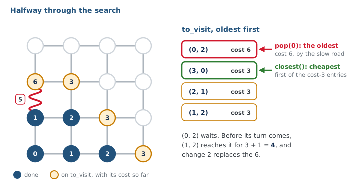
BFS takes intersections off to_visit in the order they went on — to_visit.pop(0)
— and that works because every step costs the same: the oldest entry is always one of
the closest. With weights that's no longer true. An intersection reached by a cheap
detour may be closer, in cost, than one that went on the list earlier by a slow road.
So Dijkstra keeps a second dictionary, distance, holding the cheapest cost found so
far to each intersection — it starts as {start: 0}, because the start costs
nothing to reach — and each time round the loop it takes the waiting intersection with
the smallest value. That lookup is closest(to_visit, distance): start by assuming the
first entry is best, loop over the rest, and keep any entry whose distance is smaller
— the same pattern as finding the biggest number in a list in Module 1, with the
comparison turned round. pop(0) did two jobs, choosing and removing; closest()
only chooses, so the line after it has to remove() the chosen one from to_visit.
Why can BFS get away with taking the oldest intersection off to_visit, and Dijkstra cannot?
Change 2 · Add the weight, and keep the cheaper way
BFS marks a neighbor the first time it sees it and never reconsiders; the first way to reach it is always a shortest way, in steps. Dijkstra adds the edge's weight to get the cost of reaching the neighbor this way, and if that beats what it already had, it updates. Compare the pencil versions of the two neighbor loops:
# for each neighbor of current:
#     only if it has no entry yet:
#         write where it came from
#         put it on the END of the list
# for each neighbor of current:
#     this way costs: current's cost
#         + weight(current, neighbor)
#     if no cost yet, OR this is cheaper:
#         write the cost
#         write where it came from
#         put it on the list, if not on it
Three things to notice. "Has no entry yet" was not in previous in BFS; now it's
not in distance, because distance is the dictionary that says whether a cost has
been found. The or is the whole of change 2: a neighbor that already has a cost gets
reconsidered, and loses its old cost and its old came-from if this way is cheaper.
And "if not on it" matters now, where it didn't in BFS: a neighbor can be reached a
second time while it is still waiting on to_visit, and it must not be listed twice.
previous[neighbor] = current is still how the path gets remembered, and the walk-back
at the end of the function is untouched. The only new idea is that previous can be
overwritten when a cheaper way turns up.
In Dijkstra, what happens when the planner reaches an intersection it has already recorded, by a cheaper route?
Activity · Make the two changes
Work on your copy, in this order, running test_three_planners() after each step.
Don't go on until the step's result matches.
- Write
closest(). Adddistance = {start: 0}to the setup and swapto_visit.pop(0)forclosest()+remove(). Harness: still 6 of 7 — the Module 5 properties all hold, and the cost case still fails, because nothing adds a weight yet. - Replace the neighbor loop with the weighted version. Harness: 7 of 7. The cost check now passes, with a five-step path where BFS printed three.
- Read all three planners' results, top to bottom. Expected: Manhattan fails the two blocked cases (it can't avoid walls) and the cost case; BFS passes everything except cost on the slow grid; Dijkstra passes everything. On the open grid with no slow edges, all three agree on every path length.
Then write a last test — test_cost_grid() — that adds the slow segment and calls
compare((0, 0), (0, 3)):
  BFS       steps: 3  cost: 7   [(0, 1), (0, 2), (0, 3)]
  Dijkstra  steps: 5  cost: 5   [(1, 0), (1, 1), (1, 2), (0, 2), (0, 3)]
Your Dijkstra path may go round a different way — up through x = 1 and back left
at (0, 2), or on to (1, 3) first — and still be right; cost 5 is what matters.
On a grid with no blocked intersections and no slow edges, how do the three planners' paths compare?
The cost grid
Dijkstra's distance dictionary is a map of how far everything is, in cost, from the
start. dijkstra_distances() is to compute_dijkstra_path() what bfs_distances() was
to compute_bfs_path() in Lesson 5-5: the setup and the search with no break and no
walk-back, returning distance itself. Write it, then add one line to
test_cost_grid():
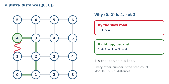
print_grid(ROWS, COLS, BLOCKED, dijkstra_distances((0, 0)))
 3 |   5  4  5  6
 2 |   4  3  4  5
 1 |   1  2  3  4
 0 |   0  1  2  3
    -------------
       0  1  2  3
Read up the left edge, x = 0: (0, 1) costs 1, then (0, 2) costs 4, not 2. The slow segment would make it 1 + 5 = 6; going over to (1, 1), up to (1, 2) and back left costs 1 + 1 + 1 + 1 = 4, so 4 is what gets kept. That one cell is change 2 doing its job. Everywhere else, the numbers are Module 5's BFS distances.
In the cost grid above, why is (0, 2) a 4 rather than a 2?
On the 4×4 floor grid one slow segment changes one number. A bigger grid shows what change 1 does to the shape of the search. Here are both searches, each following its own rule, on the 8 by 6 grid from Lesson 5-1, with a slow road through one of the two ways past the wall.
If you built the BFS class in Lesson 5-5, the copy you make is of the class: Lesson
6-5 is this lesson's class-track version, with the same two changes inside
compute_path(), and you can do it now in place of the function version. Your harness
lines are the object ones from Lesson 5-6's extension, and dijkstra_distances()
stays a function that reads planner.blocked and planner.weight(), as bfs_distances()
reads planner.blocked.
Real-world connections
1956
Edsger Dijkstra designed this in about twenty minutes, in his head, in a cafe, as a demonstration for a new computer. It is still the standard.
Under every route
Map apps run Dijkstra's algorithm (and descendants of it) over road networks with millions of weighted edges.
Upgrade by diff
Changing two lines of tested code and re-running the tests is how most real improvements ship. The copy you kept is the rollback.
Wrap-up
- What are the two changes? (Closest first; add the weight and keep the cheaper total.)
- What is
distance? (The cheapest cost found so far to each intersection.) - Where do the three planners disagree? (Walls split off Manhattan; weights split BFS from Dijkstra.)