Lesson 6-4 · Drive It
Lesson 6-4 · Drive It
Teacher mode is on. Toggle it off (bottom-right) to preview the student view.
Two planners, one grid, one trip. The robot drives from (0, 0) to (0, 3) planned by
BFS, and then the same trip planned by Dijkstra, and the class times both. BFS takes
fewer steps. Dijkstra arrives first. Nothing about the driving changes — it is Module
4's drive_path(), with the planner's name the only Module 6 line in the test.
Learning Objectives
By the end of this lesson you will be able to:
- Type a measured slow segment into the program as a setting and hand it to
add_slow_edge() - Swap the planner by changing one name, and print both planners' paths and costs before the button
- Time two runs and relate the seconds to the costs the program printed
- Explain why the driving functions did not change
This lesson's skeleton
Paste this at the end of the DIJKSTRA PLANNER section. Two settings and the outline of one driving test.
# --- Lesson 6-4: drive it ---
# The slow grid on the floor. One test, run twice:
# PLANNER_NAME picks BFS or Dijkstra, both plans are printed
# before the button, and the NAVIGATOR's drive_path() drives
# whichever was picked while the program times it. Nothing
# that drives changed: a path is a list, whoever planned it.
SLOW_SEGMENT = ((0, 1), (0, 2), 5)   # what you measured in 6-1
PLANNER_NAME = "BFS"                  # or "Dijkstra"

def test_drive_slow_grid():
    # 1. clear the slow list; add SLOW_SEGMENT to it
    # 2. position (0, 0), heading 0, destination (0, 3)
    # 3. planner = the function PLANNER_NAME names
    # 4. compare() both plans, so the choice is on screen
    # 5. plan with planner, then board.wait_for_button()
    # 6. note the time; drive_path(); note the time again
    # 7. print PLANNER_NAME, the seconds and the step count
    pass
One name changes
SLOW_SEGMENT is one tuple holding the two ends and the weight, so it can be typed in
once and handed to add_slow_edge() as SLOW_SEGMENT[0], SLOW_SEGMENT[1],
SLOW_SEGMENT[2] — the same indexing as Lesson 4-4's positions. Then the test chooses
its planner by name:
    if PLANNER_NAME == "Dijkstra":
        planner = compute_dijkstra_path
    else:
        planner = compute_bfs_path
planner = compute_dijkstra_path is the Lesson 5-6 swap: a function handed around by
name, with no parentheses. From that line on, planner(position, destination) is
whichever one was chosen, and drive_path() is handed the list it returns with no idea
which planner produced it.
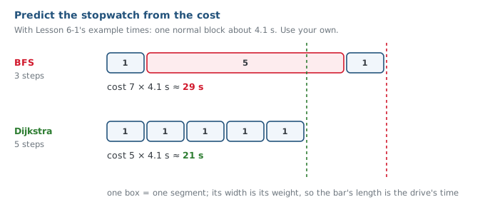
Before the button, the test calls compare() — so both plans, with their step counts
and costs, are on the screen before either run happens:
  BFS       steps: 3  cost: 7   [(0, 1), (0, 2), (0, 3)]
  Dijkstra  steps: 5  cost: 5   [(1, 0), (1, 1), (1, 2), (0, 2), (0, 3)]
Then the usual two presses: the one in RUN starts the test and prints the plans; the
one in the test is go. The timing is time.time() just before drive_path() and
just after, the difference being the seconds the drive took — a check on the stopwatch.
How much of the driving code changes between the BFS run and the Dijkstra run?
If you built the Navigator class, drive_path() is navigator.drive_path(path) with
no pose to assign back, and the plans are made from
navigator.position. If you built the planner classes and have done Lesson 6-5,
PLANNER_NAME chooses between BFS() and Dijkstra() — see that lesson.
Activity · Two runs, one stopwatch
- Write
test_drive_slow_grid()from the outline. Type your measured slow segment intoSLOW_SEGMENT, set the run line to the test, and run it with the robot on the desk: read the two printed plans and check the costs match what you worked out on paper in Lesson 6-1. Don't press the second button yet. Don't go on until the printed costs are right. PLANNER_NAME = "BFS". Robot at (0, 0) facing North on the slow grid. Run, read the printed path, press the button, start a stopwatch with the robot. Record the time. Watch it take the slow road.PLANNER_NAME = "Dijkstra". Same start, same destination. Record the time. Watch it go round.- Fill in the table:
Planner    steps   cost   seconds
BFS         ___    ___     ___
Dijkstra    ___    ___     ___
The program's own elapsed time is a check on your stopwatch. The two should tell the same story: more steps, fewer seconds.
A team's Dijkstra run takes 5 steps and 21 seconds; their BFS run takes 3 steps and 29 seconds. A normal block is about 4 seconds. Do the numbers make sense?
Both runs produce the same path and the same time. What is the most likely cause?
Real-world connections
The long way that's quicker
A map app routing you onto the highway for three extra miles is this run, at scale: more distance, less time.
Predict, then measure
Writing down the expected time before the run, from the cost, is the same discipline as writing the expected path before running a test.
Swappable planners
Real robot stacks run several planners behind one interface and switch by configuration, not by rewriting the driver.
Wrap-up
- What is the one Module 6 line in the driving test? (Which planner
planneris set to.) - What predicted the stopwatch? (The cost column.)
- Why did the robot's driving code not change? (It drives lists; it never knew what a path meant.)